📘 Traveling Salesperson Problem (TSP)
1️⃣ Introduction
The Traveling Salesperson Problem (TSP) is one of the most well-known problems in computer science, graph theory, and combinatorial optimization.
It is widely used to explain:
- Backtracking
- Branch-and-Bound
- Dynamic Programming
- NP-Complete problems
2️⃣ Problem Statement
Given:
- A set of n cities
- A distance (or cost) matrix where
C[i][j]represents the cost of traveling from city i to city j
Objective:
Find the minimum cost tour such that:
- Each city is visited exactly once
- The salesperson returns to the starting city
3️⃣ Graph Representation
- Cities → Vertices
- Paths → Edges
- Edge weights → Distance or cost
TSP can be represented using:
- Complete weighted graph
- Directed or undirected graph
4️⃣ Nature of the Problem
- Optimization problem
- Decision version is NP-Complete
- Optimization version is NP-Hard
📌 No known polynomial-time algorithm exists for TSP.
5️⃣ Approaches to Solve TSP
🔹 1. Brute Force Method
- Try all possible permutations of cities
- Select minimum cost tour
Time Complexity:
[
O(n!)
]
✔ Guarantees optimal solution
✖ Not practical for large n
🔹 2. Backtracking Approach
- Build tour incrementally
- Prune paths when cost exceeds current best
Time Complexity:
- Worst case: O(n!)
- Much faster in practice due to pruning
🔹 3. Branch-and-Bound Approach
- Use lower bound to prune unpromising tours
- Always expand the node with least cost
Time Complexity:
- Worst case: O(n!)
- Efficient for moderate values of n
🔹 4. Dynamic Programming (Held–Karp Algorithm)
Key Idea:
- Use subsets of cities
- Store intermediate results
Time Complexity:
[
O(n^2 \cdot 2^n)
]
Space Complexity:
[
O(n \cdot 2^n)
]
✔ Guarantees optimal solution
✖ Exponential space
6️⃣ TSP Using Backtracking (Concept)
🔹 Steps
- Start from city 0
- Visit unvisited cities one by one
- Accumulate path cost
- If cost ≥ best cost → backtrack
- Return to start after visiting all cities
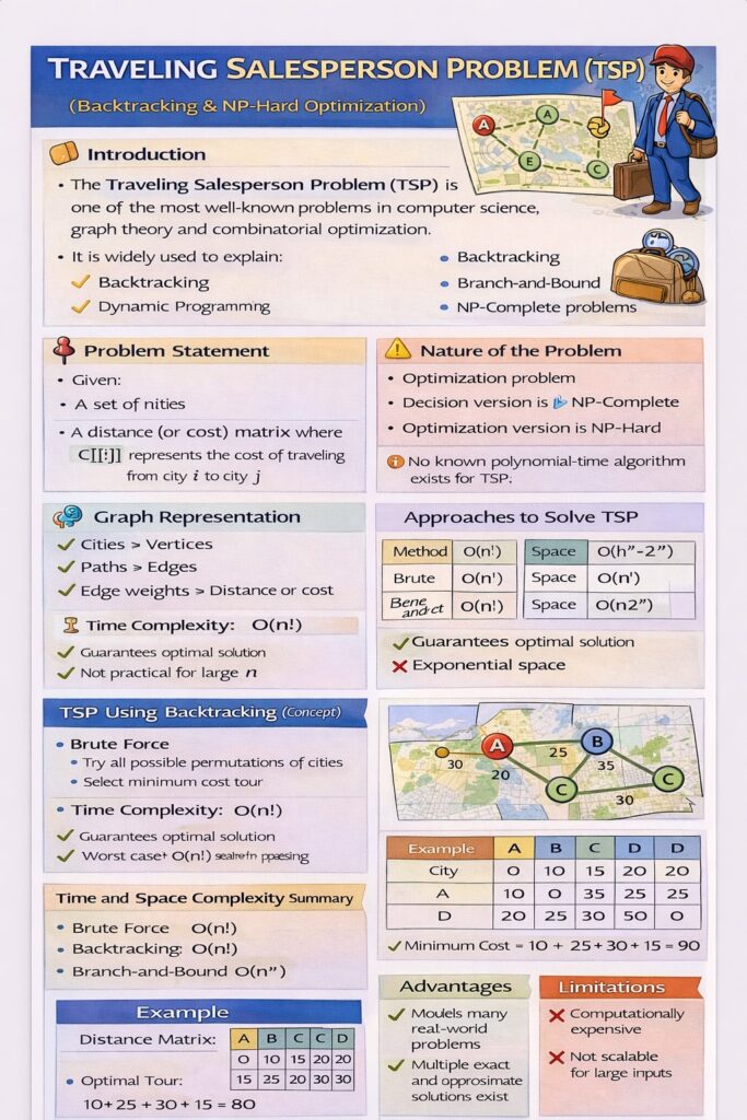
7️⃣ Example
Distance Matrix:
| City | A | B | C | D |
|---|---|---|---|---|
| A | 0 | 10 | 15 | 20 |
| B | 10 | 0 | 35 | 25 |
| C | 15 | 35 | 0 | 30 |
| D | 20 | 25 | 30 | 0 |
🔹 Optimal Tour:
A → B → D → C → A
🔹 Minimum Cost:
10 + 25 + 30 + 15 = 80
8️⃣ Time and Space Complexity Summary
| Method | Time Complexity | Space Complexity |
|---|---|---|
| Brute Force | O(n!) | O(n) |
| Backtracking | O(n!) | O(n) |
| Branch-and-Bound | O(n!) | O(n!) |
| Dynamic Programming | O(n²2ⁿ) | O(n2ⁿ) |
9️⃣ Applications of TSP
- Route planning and logistics
- Airline scheduling
- Circuit board design
- Robotics path planning
- DNA sequencing
- Network optimization
🔟 Advantages and Limitations
✔ Advantages
- Models many real-world problems
- Multiple exact and approximate solutions exist
✖ Limitations
- Computationally expensive
- Not scalable for large inputs
🔚 Conclusion
The Traveling Salesperson Problem is a cornerstone problem in algorithm design that highlights the challenges of NP-Hard optimization problems.
TSP seeks the shortest possible tour that visits each city exactly once and returns to the start.